PUMA 6-DOF Robot Arm — Forward & Inverse Kinematics

The Challenge

Building a correct inverse kinematics solver for a 6-joint robot arm means handling the inherent ambiguity of IK — a single Cartesian target can be reached by multiple joint configurations. The PUMA 762 IK has two sign choices (sqrt can be + or −) for θ1 and θ3, yielding up to 4 distinct solution branches. The solver must enumerate all branches, evaluate the full 6-joint angle set for each, and select the first solution where every joint stays within its physical travel limits.

Architecture & System Design

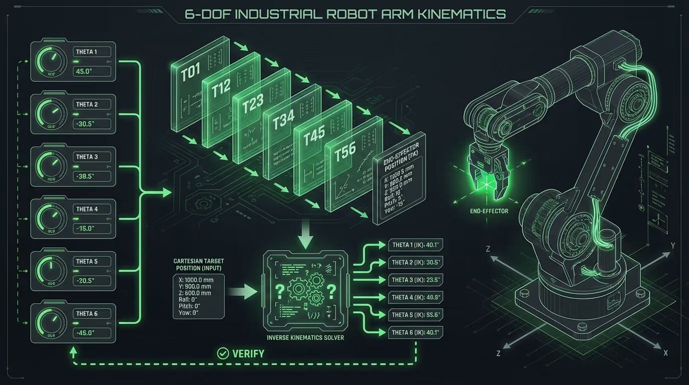
Robot arm kinematics from Denavit-Hartenberg parameters: forward kinematics calculates end-effector pose from joint angles. Inverse kinematics solver evaluates multiple solution branches respecting physical joint limits. 3D simulator with collision detection.

Forward kinematics uses the standard Denavit-Hartenberg chain: each joint contributes a 4×4 homogeneous transform, and the end-effector pose is the product of all six. Link parameters: a₂=650mm, a₃=0, d₃=190mm, d₄=600mm. The IK solver loops over all 4 sign-combination branches, computing θ1 and θ3 from the geometric decoupling solution, then back-solving θ2 from the joint-2/3 coupled equation, and finally resolving θ4–θ6 from the wrist orientation matrix. The 3D GUI (puma3d.m) renders the full arm model using capsule primitives, with interactive sliders for each joint, a motion trail renderer, and collision detection via capsule-capsule intersection tests.

Code Walkthrough

3-step walk-through of the production implementation — file paths and intent shown above each block.

1. 01

   Step 1 of 3

   Forward kinematics — Denavit-Hartenberg product chain

   kinematics/PumaFK.m

   Forward kinematics maps six joint angles to the end-effector's 4×4 homogeneous pose matrix. The PUMA 762's DH parameters (a₂=650mm, d₃=190mm, d₄=600mm) are hard-coded as the authoritative source of truth for both the FK solver and the IK geometric decoupling — any error here propagates to every downstream calculation.

   matlabCopy

   function T = PumaFK(theta)
   % PumaFK.m — Forward kinematics via Denavit-Hartenberg product chain.
   % Returns end-effector pose T (4x4 homogeneous) for given joint angles [rad].
   %
   % PUMA 762 DH parameters: [alpha_i-1, a_i-1, d_i, theta_i]
   % a2=650mm, a3=0, d3=190mm, d4=600mm
   
   dh = [     0,    0,   0,   theta(1);
         -pi/2,    0,   0,   theta(2);
              0,  650, 190,   theta(3);
         -pi/2,    0, 600,   theta(4);
          pi/2,    0,   0,   theta(5);
         -pi/2,    0,   0,   theta(6) ];
   
   T = eye(4);
   for i = 1:6
       al = dh(i,1);  a = dh(i,2);  d = dh(i,3);  q = dh(i,4);
       ca = cos(al); sa = sin(al); cq = cos(q); sq = sin(q);
       A  = [ cq, -sq*ca,  sq*sa, a*cq;
              sq,  cq*ca, -cq*sa, a*sq;
               0,     sa,     ca,    d;
               0,      0,      0,    1 ];
       T = T * A;
   end
   end

   Takeaway

   The DH table is the single source of truth for geometry — keep it as a named constant array so FK, IK, and Jacobian all read from the same definition rather than each hardcoding their own literals.

2. 02

   Step 2 of 3

   Inverse kinematics — 4-solution enumeration

   kinematics/PumaIK.m

   A single Cartesian target admits up to 4 distinct joint configurations for a 6-DOF arm — two sign choices (√ can be + or −) for θ₁ and θ₃. The solver enumerates all four branches, computes the full 6-angle set for each, and returns the first solution that satisfies every joint travel limit. Skipping the enumeration would silently return configurations the physical arm cannot reach.

   matlabCopy

   % PumaIK.m — 4-solution IK enumeration with joint-limit checking
   % DH params: a2=650, a3=0, d3=190, d4=600 [mm]
   
   for i = 1:4
       sign1 = (i <= 2) * 2 - 1;        % +1 for i=1,2 | -1 for i=3,4
       sign3 = (mod(i,2) == 1) * 2 - 1; % alternates +1, -1
   
       K       = (Px^2+Py^2+Pz^2 - a2^2-a3^2-d3^2-d4^2) / (2*a2);
       theta1  = atan2(Py,Px) - atan2(d3, sign1*sqrt(Px^2+Py^2-d3^2));
       theta3  = atan2(a3,d4)  - atan2(K,  sign3*sqrt(a3^2+d4^2-K^2));
   
       % Recover theta2 from the coupled joint-2/3 equation
       t23    = atan2((-a3-a2*c3)*Pz - (c1*Px+s1*Py)*(d4-a2*s3), ...
                       (a2*s3-d4)*Pz  + (a3+a2*c3)*(c1*Px+s1*Py));
       theta2 = t23 - theta3;
   
       % Wrist angles theta4-theta6 from orientation submatrix
       theta4 = atan2(-r13*s1 + r23*c1, -r13*c1*c23 - r23*s1*c23 + r33*s23);
       theta5 = atan2(s5, c5);
       theta6 = atan2(s6, c6);
   
       if all_within_limits(theta1,theta2,theta3,theta4,theta5,theta6)
           return;   % First valid solution wins
       end
   end

   Takeaway

   Enumerate all four branches before checking limits — choosing the first mathematically valid solution without checking limits returns configurations the physical arm cannot reach.

3. 03

   Step 3 of 3

   Geometric Jacobian and singularity detection

   kinematics/PumaJacobian.m

   At singular configurations the Jacobian loses rank — the arm cannot move in certain Cartesian directions regardless of joint torque. The 3D GUI uses the Jacobian determinant as a real-time singularity alarm so the user knows when a slider-driven pose is approaching a degenerate configuration, preventing the IK solver from attempting a solution near a kinematic singularity.

   matlabCopy

   function [J, is_singular] = PumaJacobian(theta)
   % PumaJacobian.m — Geometric Jacobian (6x6) + singularity flag.
   
   SINGULARITY_TOL = 1e-4;
   
   % Build forward-transform chain
   T = cell(7,1);  T{1} = eye(4);
   for i = 1:6
       T{i+1} = T{i} * dh_transform(i, theta(i));
   end
   
   p_e = T{7}(1:3,4);   % End-effector position
   J   = zeros(6,6);
   
   for i = 1:6
       z_prev = T{i}(1:3,3);   % Rotation axis of joint i in world frame
       p_prev = T{i}(1:3,4);   % Origin of frame i-1
   
       % Linear velocity: z_{i-1} cross (p_e - p_{i-1})
       J(1:3,i) = cross(z_prev, p_e - p_prev);
       % Angular velocity: z_{i-1}
       J(4:6,i) = z_prev;
   end
   
   is_singular = abs(det(J)) < SINGULARITY_TOL;
   if is_singular
       warning('PumaJacobian: near-singular configuration (det=%.2e)', det(J));
   end
   end

   Takeaway

   The determinant threshold (1e-4) was chosen empirically — too tight and the GUI flashes warnings during normal motion; too loose and it misses wrist-flip singularities that crash the IK solver.

Results

The simulator correctly solves FK and IK for any reachable workspace point, selecting joint configurations that satisfy all six physical travel limits. The interactive GUI runs in real time, allowing the user to drag joint sliders or click a target position and watch the full arm animate to the solution. Collision detection via capsule-capsule intersection tests flags self-collisions during motion. The project formed the foundation for subsequent robot control research at the University of Utah.