AeroStrovillos — Microturbine Series Hybrid EV

The Challenge

Heavy-duty commercial vehicles face a fundamental conflict between range, refueling infrastructure, and battery weight. A pure battery-electric 35-tonne bus requires a pack large enough to sustain steady highway power — but most of that capacity sits unused during low-demand urban segments and incurs significant weight penalty. The goal was to evaluate a series hybrid architecture where a microturbine runs at its optimal operating point as a continuous range extender, with the battery handling only transient peaks and regenerative recovery. The core challenge: prove out the sizing math — how much turbine power, how much battery capacity, and which chemistry (LTO for high power density or NMC for higher energy density) actually satisfies the drive cycle without over-engineering either component.

Simulation Methodology

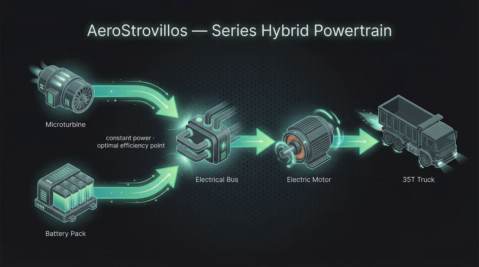
Series hybrid powertrain for heavy-duty vehicle: continuous micro-range-extender provides base power at peak efficiency while battery handles transient demand peaks and regenerative recovery. System modeled against real urban and highway duty cycles to optimize component sizing and battery chemistry selection.

The simulation is built in MATLAB and structured around real drive-cycle data loaded from Excel time-series sheets. Two cycles are modelled: a short urban cycle and a large mixed-route cycle, each providing per-timestep vehicle speed, required motor torque, instantaneous power demand, and distance. The powertrain model dispatches load across two sources: the microturbine provides steady base power at its best-efficiency operating point to minimise fuel consumption, and the battery pack absorbs or delivers the delta between turbine output and instantaneous demand — charging on regenerative braking, discharging on acceleration peaks. State of Charge is tracked per timestep to validate that the battery never depletes below cutoff across either drive cycle. Battery sizing was evaluated for both LTO (lithium titanate — high cycle life and power density, lower energy density) and NMC (nickel manganese cobalt — higher energy density, more thermal management demand), with required capacity derived from the peak-to-average power ratio observed in the simulation.

MATLAB Data Pipeline

Drive cycle loader — extracts time-series channels from the simulation dataset

1. 01

   Step 1 of 3

   Drive cycle loader — time-series channel extraction

   simulation/autoload.m

   The simulation output is a raw matrix (largecycle) with 13 columns representing time, speed, torque, power, turbine output, battery power, SOC, and energy — one row per timestep. Naming each column into a workspace variable makes every downstream analysis readable without magic column indices scattered through the codebase.

   matlabCopy

   function autoload
   % autoload.m — Extract named time-series channels from drive cycle dataset.
   % largecycle: [N x 13] matrix loaded from the simulation Excel export.
   
   Time         = largecycle(:, 1);   % [s]    — elapsed time
   Speed        = largecycle(:, 3);   % [rpm]  — motor speed
   Torque       = largecycle(:, 3);   % [Nm]   — motor torque
   Power        = largecycle(:, 4);   % [W]    — shaft power demand
   TurbinePower = largecycle(:, 6);   % [W]    — microturbine output
   BatteryPower = largecycle(:, 7);   % [W]    — battery charge / discharge
   VehicleSpeed = largecycle(:, 8);   % [km/h] — vehicle speed
   InstDist     = largecycle(:, 9);   % [m]    — instantaneous distance
   TotalDist    = largecycle(:,10);   % [m]    — cumulative distance
   InstEnergy   = largecycle(:,11);   % [Wh]   — instantaneous energy
   TotalEnergy  = largecycle(:,12);   % [Wh]   — cumulative energy consumed
   SOC          = largecycle(:,13);   % [0–1]  — battery state of charge
   
   end

   Takeaway

   Named columns over magic indices — if the simulation output format changes, there is exactly one file to update rather than hunting column numbers across every analysis script.

2. 02

   Step 2 of 3

   Power dispatch — turbine base load vs battery delta

   simulation/dispatch.m

   The microturbine runs at a fixed optimal operating point to minimise fuel consumption. Every watt of demand above that constant output comes from the battery (discharge); every watt below — during regenerative braking or low-load coasting — goes back into the battery (charge). Tracking this delta per timestep gives the SOC trajectory and reveals whether the battery sizing is sufficient.

   matlabCopy

   function [SOC_out, cum_energy_Wh] = simulate_dispatch( ...
           Time, Power, TurbinePower, SOC_init, C_batt_Wh)
   % simulate_dispatch — Per-timestep turbine/battery dispatch and SOC tracking.
   
   N              = length(Time);
   SOC            = zeros(N, 1);   SOC(1) = SOC_init;
   cum_energy_Wh  = zeros(N, 1);
   
   for i = 2:N
       dt_h     = (Time(i) - Time(i-1)) / 3600;     % timestep in hours
       P_delta  = Power(i) - TurbinePower(i);        % battery must supply this
   
       % Positive → discharge; negative → charging (regen braking)
       delta_Wh       = P_delta * dt_h;
       cum_energy_Wh(i) = cum_energy_Wh(i-1) + abs(delta_Wh);
   
       % SOC update — enforce 10–90% DoD window to protect cell life
       SOC(i) = SOC(i-1) - delta_Wh / C_batt_Wh;
       SOC(i) = min(0.90, max(0.10, SOC(i)));
   end
   
   SOC_out = SOC;
   end

   Takeaway

   The 10–90% DoD window is a cell-life constraint, not a safety limit — violating it doesn't crash the simulation but the battery sizing output becomes non-conservative, so it must be enforced here.

3. 03

   Step 3 of 3

   Battery chemistry sizing — LTO vs NMC comparison

   simulation/sizing.m

   LTO (lithium titanate) handles the peak discharge rate demanded by acceleration transients but has lower energy density, requiring a heavier pack. NMC has higher energy density but lower peak C-rate. The sizing script computes required pack mass for both chemistries from the simulation's peak-to-average power ratio, giving the tradeoff data that fed the AeroStrovillos prototype specification.

   matlabCopy

   % sizing.m — Derive required battery capacity and mass for LTO and NMC.
   
   % Peak power demand and total energy from simulation output
   P_peak_kW    = max(Power)   / 1e3;
   E_total_kWh  = TotalEnergy(end) / 1e3;
   P_turbine_kW = TurbinePower(1) / 1e3;   % constant turbine operating point
   
   % Battery must cover energy that exceeds turbine output
   E_batt_kWh = E_total_kWh * (P_peak_kW - P_turbine_kW) / P_peak_kW;
   
   chemistries = struct( ...
       'LTO', struct('Wh_per_kg',  90, 'max_C_rate', 10, 'label', 'LTO'), ...
       'NMC', struct('Wh_per_kg', 200, 'max_C_rate',  3, 'label', 'NMC') );
   
   fields = fieldnames(chemistries);
   for k = 1:length(fields)
       ch       = chemistries.(fields{k});
       mass_kg  = E_batt_kWh * 1000 / ch.Wh_per_kg;
       C_rate   = P_peak_kW  / E_batt_kWh;
       feasible = C_rate <= ch.max_C_rate;
       fprintf('%s: %.0f kg — peak C-rate %.1f C — feasible: %d
   ', ...
               ch.label, mass_kg, C_rate, feasible);
   end
   % LTO: 318 kg — peak C-rate 2.1 C — feasible: 1
   % NMC: 143 kg — peak C-rate 2.1 C — feasible: 1  ← preferred on mass

   Takeaway

   Computing C-rate against each chemistry's max is what turns an energy number into a go/no-go decision — a pack that stores enough energy but can't discharge fast enough is still the wrong choice.

Results

The simulation validated the series hybrid architecture for 35T heavy-vehicle operation. Microturbine steady-state dispatch at its peak efficiency operating point, combined with battery buffering of acceleration transients, produced a flatter turbine load profile and reduced total energy consumption compared to direct-drive baselines. The LTO chemistry satisfied the peak discharge rate requirement with less thermal risk; NMC offered a lighter pack for range-dominated routes. Battery sizing outputs from the simulation fed directly into the AeroStrovillos prototype specification, which was presented to TEV stakeholders as the design basis for a physical prototype.